Multi-dimensional Indexing in Numpy
(This post is based on a StackOverflow answer)
What is tuple-indexing in Numpy?
If you want to index an element in a multi-dimensional (i.e. nested) list in Python, you have to do this manually:
>>> nested_list = [
...     [1, 2, 3],
...     [4, 5, 6],
...     [7, 8, 9],
... ]
>>> print(nested_list[1][1])
5
This is already ugly for this 2-dimensional example, and for lists that have more levels of nesting it only gets worse.
Numpy is a great python package for working with multi-dimensional numerical data. You can effectively use it the same as if it is still the same data-structure in Python.
>>> import numpy as np
>>> nested_array = np.array([
...     [1, 2, 3],
...     [4, 5, 6],
...     [7, 8, 9],
... ])
>>> print(nested_array[1][1])
5
However, Numpy also natively supports tuple-indexing:
>>> print(nested_array[(1, 1)])
5
>>> print(nested_array[1, 1])
5
So… which is faster?
Simple experiments: 1D, 2D and now also in 3D!
Let’s start with the 1D case to get a baseline:
A = np.zeros(8)
%timeit A[4]
183 ns ± 3 ns per loop (mean ± std. dev. of 7 runs, 10000000 loops each)
Indexing a single value in a single-dimensional array takes just under 200 nanoseconds on my laptop. Now let’s see how that time scales to two-dimensional arrays.
A = np.zeros((8,8))
%timeit A[4][4]
373 ns ± 6.12 ns per loop (mean ± std. dev. of 7 runs, 1000000 loops each)
%timeit A[4, 4]
202 ns ± 2.42 ns per loop (mean ± std. dev. of 7 runs, 1000000 loops each)
As you can see, using numpy’s tuple-indexing is still around 200 nanoseconds, while using list-indexing takes about twice as long!
What is probably happening, is that each A[x] is translated to A.__getitem__(x). This means that when x is a tuple, it is passed down to numpy’s own functions to handle the multi-dimensional indexing. But when using list-indexing, this is executed as a nested call to the __getitem__ method. For the 2D case we just tested, this results in
(A.__getitem__(4)).__getitem__(4)
where each __getitem__ takes ~200 nanoseconds as we’ve seen before. So for a 3D array, we expect numpy’s tuple-indexing to be constant-time, while list-indexing scales linearly:
A = np.zeros((8, 8, 8))
%timeit A[4][4][4]
614 ns ± 17.4 ns per loop (mean ± std. dev. of 7 runs, 1000000 loops each)
%timeit A[4, 4, 4]
236 ns ± 14.4 ns per loop (mean ± std. dev. of 7 runs, 1000000 loops each)
Yep, that’s about what we expected: just over 200 nanoseconds for the tuple-indexing, and three times that for the list-indexing.
Extended experiments up to 10D
To make sure we’re getting the full picture, let’s repeat the previous experiments all the way up to 10-dimensional arrays. We’ll reduce the size in each dimension to 4 to make sure Python doesn’t return a MemoryError when allocating the array.
The following script times the same indexing statement we’ve tested previously, and passes along the locally created array A to the globals parameter as an alternative to defining it as setup.
By using min(repeat(...)) instead of timeit(...) we get the minimum time out of 5 runs. This means our results are less likely influenced by any other processes that happen to be running at the same time during our script.
These experiments make heavy use of the Python 3.6+ f-strings. For more information on them, see here or let me know if you want me to write a blog post about them
from timeit import repeat
import matplotlib.pyplot as plt

list_idxing = []
tupl_idxing = []
ndims = range(1, 11)
for ndim in ndims:
    A = np.zeros([4]*ndim)
    list_idxing.append(
        min(repeat(f"A{'[2]'*ndim}", globals={'A': A}))
    )
    tupl_idxing.append(
        min(repeat(f"A[{','.join(['2']*ndim)}]", globals={'A': A}))
    )

plt.plot(ndims, list_idxing, label='list indexing')
plt.plot(ndims, tupl_idxing, label='tuple indexing')
plt.xlabel("Number of dimensions")
plt.ylabel("Microseconds per loop")
plt.legend(loc=0)
plt.show()
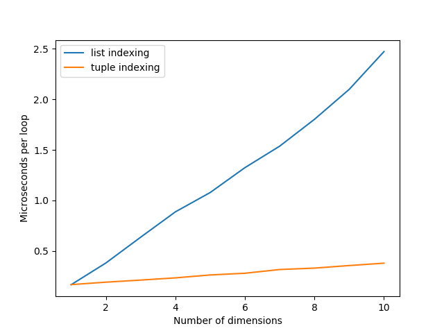
The resulting graph does indeed show that the time of tuple-indexing remains roughly constant, while list-indexing keeps growing linearly.
We have created the arrays to be increasingly larger for each of the above timings. To rule out whether that has any effect, we can repeat the experiments with the largest array already allocated, and just index the relevant slices from them:
list_idxing = []
tupl_idxing = []
B = np.zeros([4]*10)
ndims = range(1, 11)
for ndim in ndims:
    list_idxing.append(
        min(repeat(f"B{'[2]'*ndim}", globals={'B': B}))
    )
    tupl_idxing.append(
        min(repeat(f"B[{','.join(['2']*ndim)}]", globals={'B': B}))
    )

plt.plot(ndims, list_idxing, label='list indexing')
plt.plot(ndims, tupl_idxing, label='tuple indexing')
plt.xlabel("Number of dimensions")
plt.ylabel("Microseconds per loop")
plt.legend(loc=0)
plt.show()
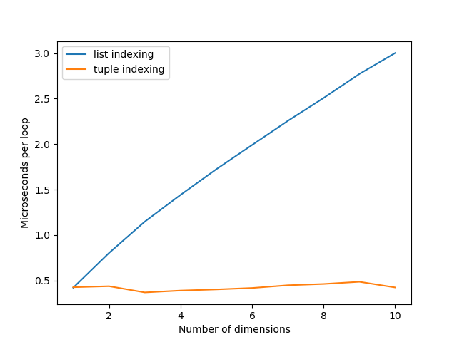
Comparing this graph to the previous one, it does seem like the time for tuple-indexing is consistently at ~500 nanoseconds now instead of slowly increasing from ~200. So there does seem to be some overhead involved that depends on the number of dimensions of the array you’re indexing.
Comparing the graphs for list-indexing, we can see a similar shift upwards in the amount of time required. The overall trend is still linearly increasing, and does not compare any more favourably against tuple-indexing.
Conclusion
Using tuple-indexing is significantly faster than nested indexing.